DeepSeek's Attention Evolution - [DSA, CSA, CSA2]
Note | Preface
This is the second post in the DeepSeek Attention evolution series. The previous one, DeepSeek’s Attention Evolution -【MLA】, covered the evolution from MHA to MLA; this post picks up with DSA, CSA and CSA2. MLA solved the storage form of the KVCache, but its compute complexity is still $O(N^2)$ and the KVCache is still $O(N)$, so it still struggles with 256K/1M long contexts. This post follows the DeepSeek V3.2-exp → V4 → V4.1-Flash line to see how it pushes the algorithmic and engineering tradeoffs to the limit, step by step, across sparse attention, KV compression and cross-layer sharing.
Caution | Disclaimer
Since I wrote this on a whim, there are inevitably some typos, especially misspelled words — feel free to point them out and help me correct them
1. Starting from MLA’s bottleneck: why we need sparse attention
Note that in real models, Sparse Attention / Linear Attention needs to be used together with Full Attention in a certain ratio, typically a hybrid of Full : Sparse = 1:3 / 1:4.
The previous post covered the evolution from MHA to MLA; this post continues with DSA and CSA. As good as MLA is, its computational complexity is still $O(N^2)$, and the space complexity of the KVCache is still $O(N)$, which falls short when facing the 256K/1M long-context scenarios that followed. So to break out of this predicament, DeepSeek started using the DeepSeek Sparse Attention structure as the main attention structure in the V3.2-exp release to solve this problem.
2 The 2-8 Rule of Attention: From MLA to DSA
2.1 Why sparsity can represent most features
In tasks that predict text sequences, we often observe a phenomenon: attention tends to concentrate on a few individual words. For example, in “I need to go to the station at 7 PM this afternoon, how should I plan my trip,” when predicting forward, the features need to focus on very high-frequency signals like “7 PM this afternoon” and “trip,” while tokens like “I” carry little signal for the features of subsequent tokens. Some tokens are very high-frequency, but attention on some tokens is relatively sparse. Based on this prior, we can use a relatively small index network to compute the most important tokens, and then only compute attention over a subset of key tokens during attention, thereby improving overall efficiency.
First, to demonstrate that “key tokens” can represent most of the overall information, I vibed a small experiment on Qwen3-0.6B. Here, “key” is defined as positions to which the current query assigns relatively high attention weights.
The experiment itself is fairly simple. I prepared six passages of text: Chinese narrative, Chinese expository, English narrative, English expository, Python code, and a passage of Chinese document retrieval content (all roughly 300 tokens). Each raw passage is fed directly into the model for a single prefill, and then the attention weights after Softmax at each layer are recorded. For a head, one row of the attention matrix indicates how much weight the current query assigns to each visible key. The statistic is computed as follows: for each row, sort the visible weights in descending order, then calculate how much attention weight is covered by keeping the top $p$ proportion of positions. Suppose the current row has $n$ visible positions, and the sorted weights are $a_{(1)}\geq a_{(2)}\geq\cdots\geq a_{(n)}$, define:
$$ C(p)=\sum_{j=1}^{\lceil pn\rceil}a_{(j)}. $$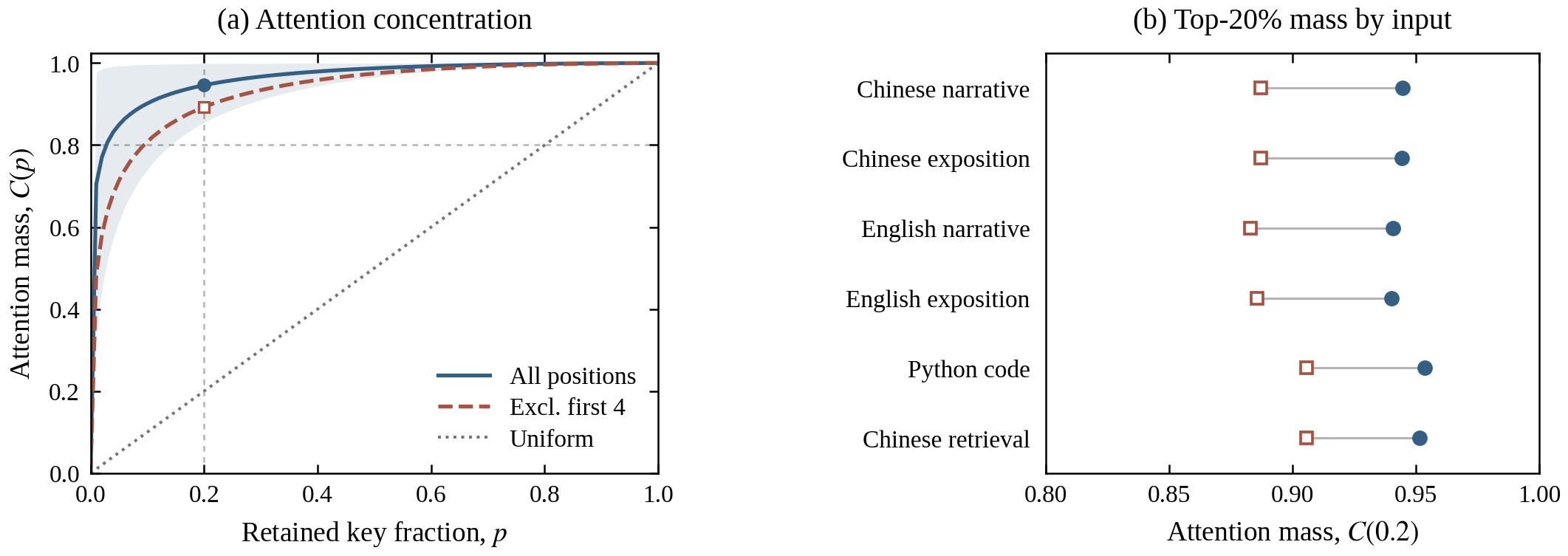
Insight | The 2-8 rule of attention
We can observe that when p=0.2 (keeping the top 20% of high-frequency attention scores), $C(p)$ on this set of inputs basically reaches above 90%. In practice, this fits the 2-8 rule commonly seen in computing, i.e., a small number of key positions provide most of the information.
2.2 Indexer+MLA=DSA
When discussing this phenomenon above, I mentioned that a group of Indexer networks could compute the high-frequency Score positions, and then during attention only mask the tokens in that part to participate in the computation. If we set the indexer to select the TopK positions, that is, $K$ positions, then the computational complexity of attention drops from $O(N^2)$ to $O(NK)$. So how does DeepSeek design DSA? First, let’s set aside the backbone — the backbone is still the MLA detailed in the previous article DeepSeek’s Attention Evolution -【MLA】. Let’s look at the Indexer. Based on our understanding of attention, we can also design the Indexer as a streamlined attention, except that, similar to MLA, we compress the Indexer’s Q/KV much more aggressively, with lower dimensions, because it only needs to compute a very rough relevance. The figure below shows the DSA Indexer structure — it’s essentially like a miniature attention, but for the sake of computational throughput1, it doesn’t choose the traditional Softmax way to compute scores; instead it directly uses ReLU+head weight to compute them. There are two reasons for choosing ReLU+weight:
- Adding Softmax after the final score doesn’t help Top-k: and since we only need to output indices, there’s no need for normalization either — just take the index via argmax directly.
- Using ReLU per head is easier to compute efficiently than doing Softmax per head: needless to say, ReLU is just a simple piecewise function, whereas Softmax requires computing transcendental functions.
Note | Softmax for training, ReLU for inference
Note that in actual training, softmax is still used, but in the end KL is used for alignment2, and at inference time ReLU+weight is used entirely.
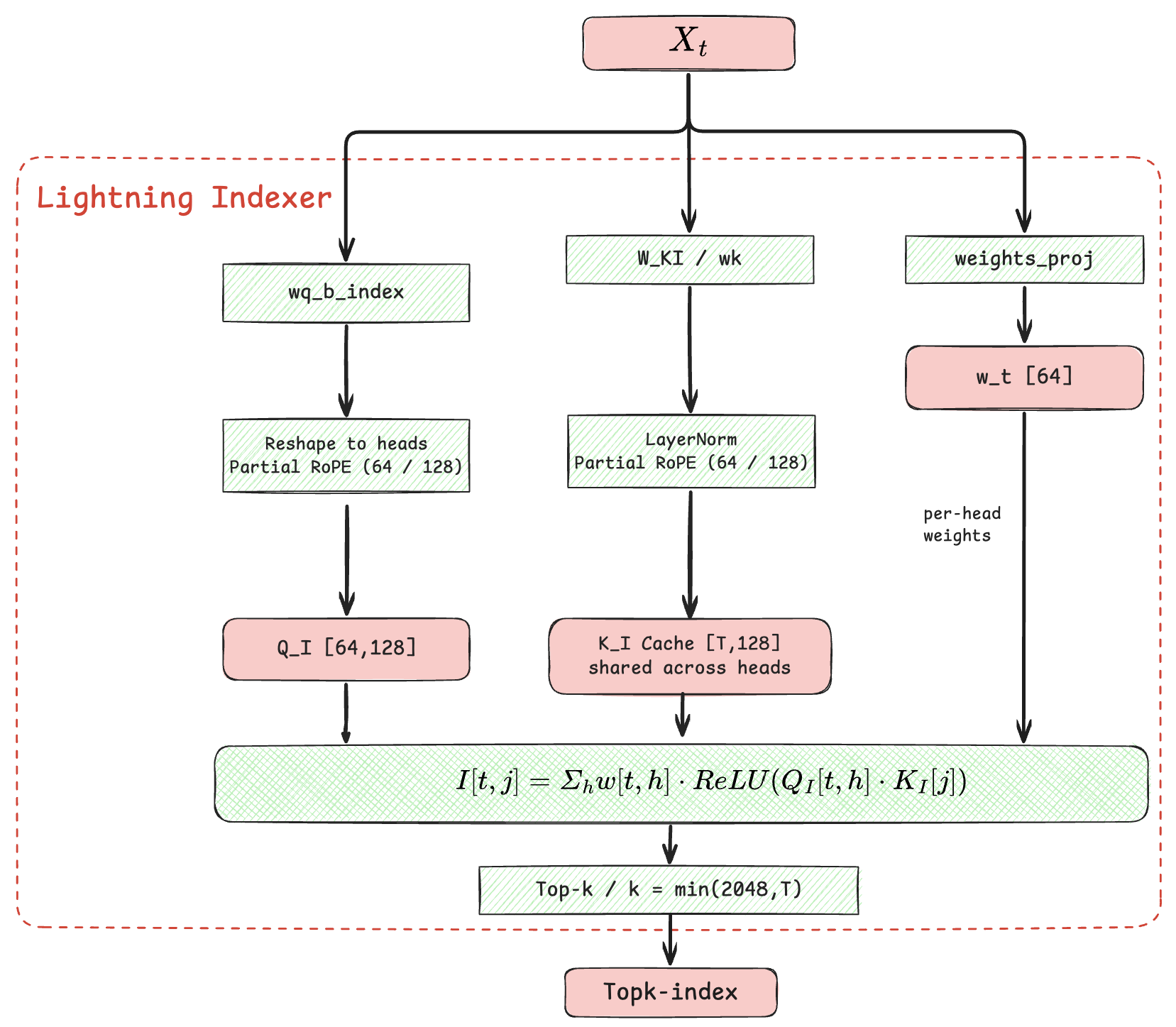
This structure is called the Lightning Indexer in DeepSeek Sparse Attention.
Combined with the previous MLA, the overall structure is DeepSeek Sparse Attention (DSA):
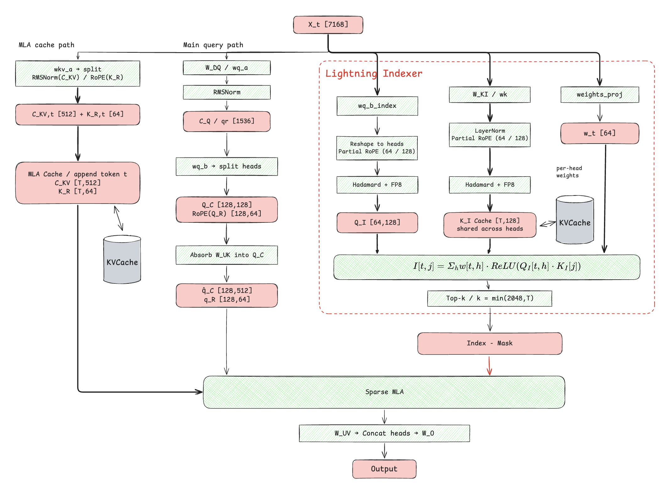
Compared with the previous pipeline, a KVCache slot is added at step $K_I$.
2.3 Kernel optimization: the algorithm’s ideal vs. engineering reality
At first glance, DSA improves efficiency both in concept and in algorithm, but in practice there are many engineering difficulties, for example:
- The conventional
torch.topkimplementation of Top-k is so inefficient that it drags down the whole implementation. - Sparse MLA does not perform as well as Dense MLA in short-context / low-concurrency settings, but in long contexts, because $K \ll L$ is far superior to the previous MLA from an algorithmic standpoint.
To solve the problems caused by Top-K, many engineering approaches have since been developed, including Radix-select-based Top-K3, Guess-Verify-Refine4, and DeepSelect5, all of which address the inefficiency of Top-k. I won’t go into detail here; I can write a separate post later specifically about the Top-K problem.
As for Sparse MLA, it is essentially still the Sparse MQA and Sparse MHA kernel, because MLA has two computation forms6, which I covered in an earlier blog post. But overall, because of the fixed overhead of $K$ and the sparse indexing problem, SM utilization is not very high in short contexts and low concurrency7, and the flashMLA blog also mentions this issue. To address sparsity and the $K$ problem, for example, trtllm skips the indexer computation in small contexts, and both vLLM and sglang have implemented this approach8, and it is enabled by default.
After all this optimization, the overall DSA structure is now very solid performance-wise, and it is widely used in other popular models, such as the GLM5.x series and MinimaxM3’s MSA9, which is a modified version built on DSA.
2.4 Can the attention positions be consistent across layers: IndexCache
Having looked at the sparse attention approach represented by DSA, does attention across layers also share the same important tokens? It turns out it does — GLM measured the token positions selected by the Indexer in adjacent layers of their DSA and found that 70% of them were the same10.
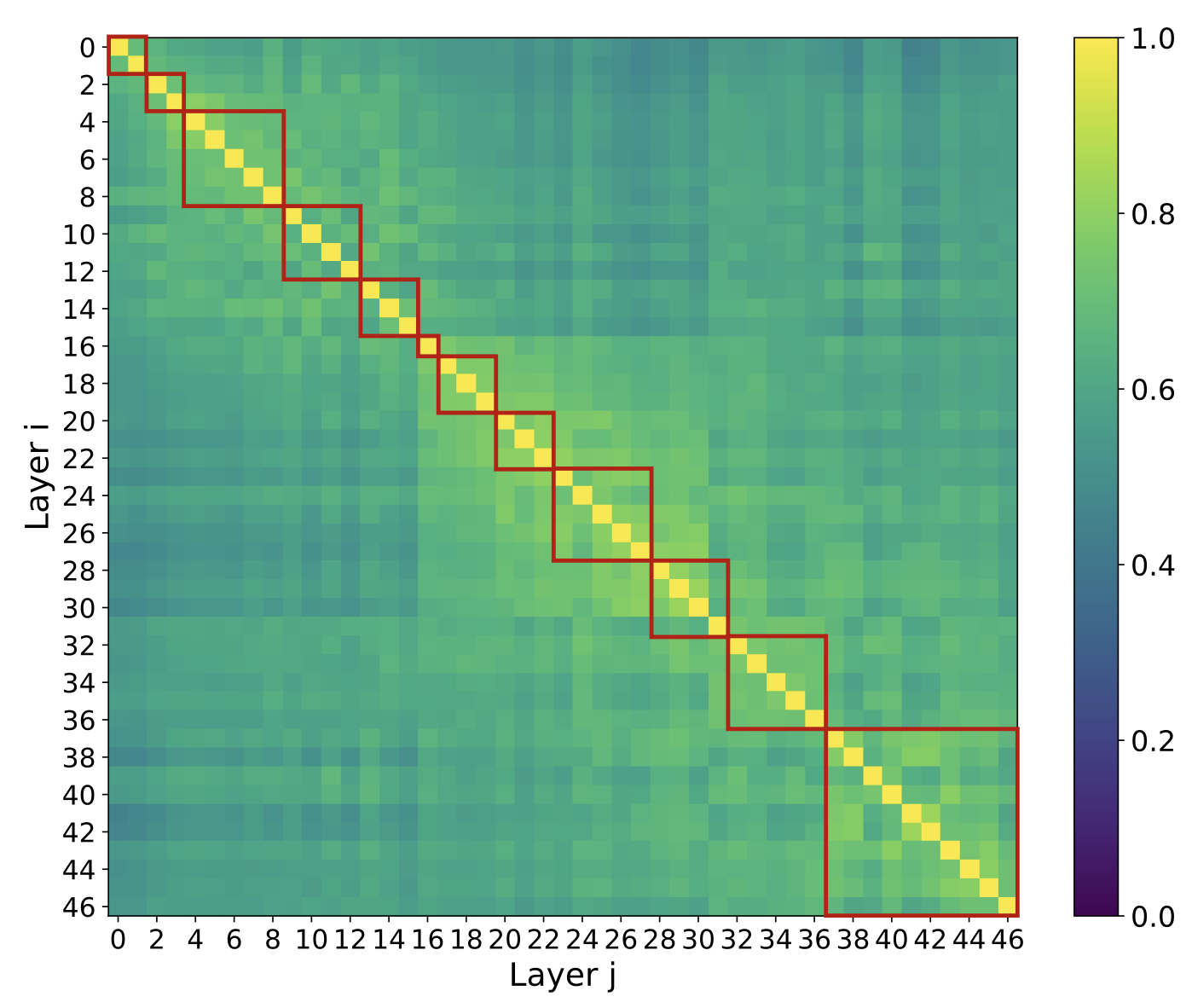
So GLM developed another acceleration method: since Top-k is relatively slow, measure the similarity between layers and cache the index of similar layers, so that layers selecting the same tokens can directly share one Indexer. Of course, this approach requires some fine-tuning, because adjacent layers are only similar, and some fine-tuning is needed to tune the Indexers of similar layers into agreement. By caching the Indexer, you can get roughly a 1.5-2x speedup. This optimization is widely used in the GLM5.x model series.
3. Combining SlidingAttention and SparseAttention: The Birth of CSA
Having read the above, the reader presumably now has some understanding of DSA. DSA solved the computational burden of long contexts, but it did not solve the pressure on the KVCache — in fact, because of the Indexer, it added one more KVCache slot, slightly increasing KVCache storage pressure.
Important | What is reduced is storage pressure, not transfer pressure
What is mentioned here is that DSA does not reduce the storage pressure of the KVCache, not the transfer pressure of the KVCache during computation — that has already been solved in DSA, because the Indexer only selects TopK positions, so the pressure of loading the KVCache is a constant.
In the V4 version, DeepSeek proposed two structures to solve the above KVCache problem:
- Compressed Sparse Attention (CSA): a combination of Sparse Attention + Sliding Attention + KVCompressor
- Heavily Compressed Attention (HCA): an extremely compressed KVCompressor followed directly by MQA.
The combination of the two is like HCA handling the global summary, with a more extreme compression ratio, while CSA handles a finer-grained skim + close read.
To add a method for compressing the KV, DeepSeek first introduced the Compressor structure, which is also the core of CSA. Through a pooling + Gate-like approach, it compresses multiple tokens into one, thereby reducing the overall KVCache storage pressure.
3.1 Gating and pooling over KV: the Compressor
The structure itself isn’t complicated. If you’re reasonably familiar with deep learning, it’s just a gated pooling, as shown below:
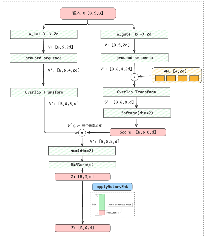
First, X is projected, then grouped by compression rate. In the example above, every 4 tokens are compressed into one, so the dimension of $V'$ is $[B,G,4,2d]$, where $G = S/4$. Since the gate needs to compute the combined weight of these 4 tokens, the gate path also needs the same projection.
The overlap transform is also a critical operation. It’s similar to the slice overlap trick we commonly use in RAG: the information in the next segment needs to overlap with the range of the previous segment, so that a single token gets a wider field of view. The overall idea is that the previous $2d$ is split into an upper half and a lower half; each entry in the upper half takes the upper half of the previous group, and then interleaves with the current lower half. As shown:
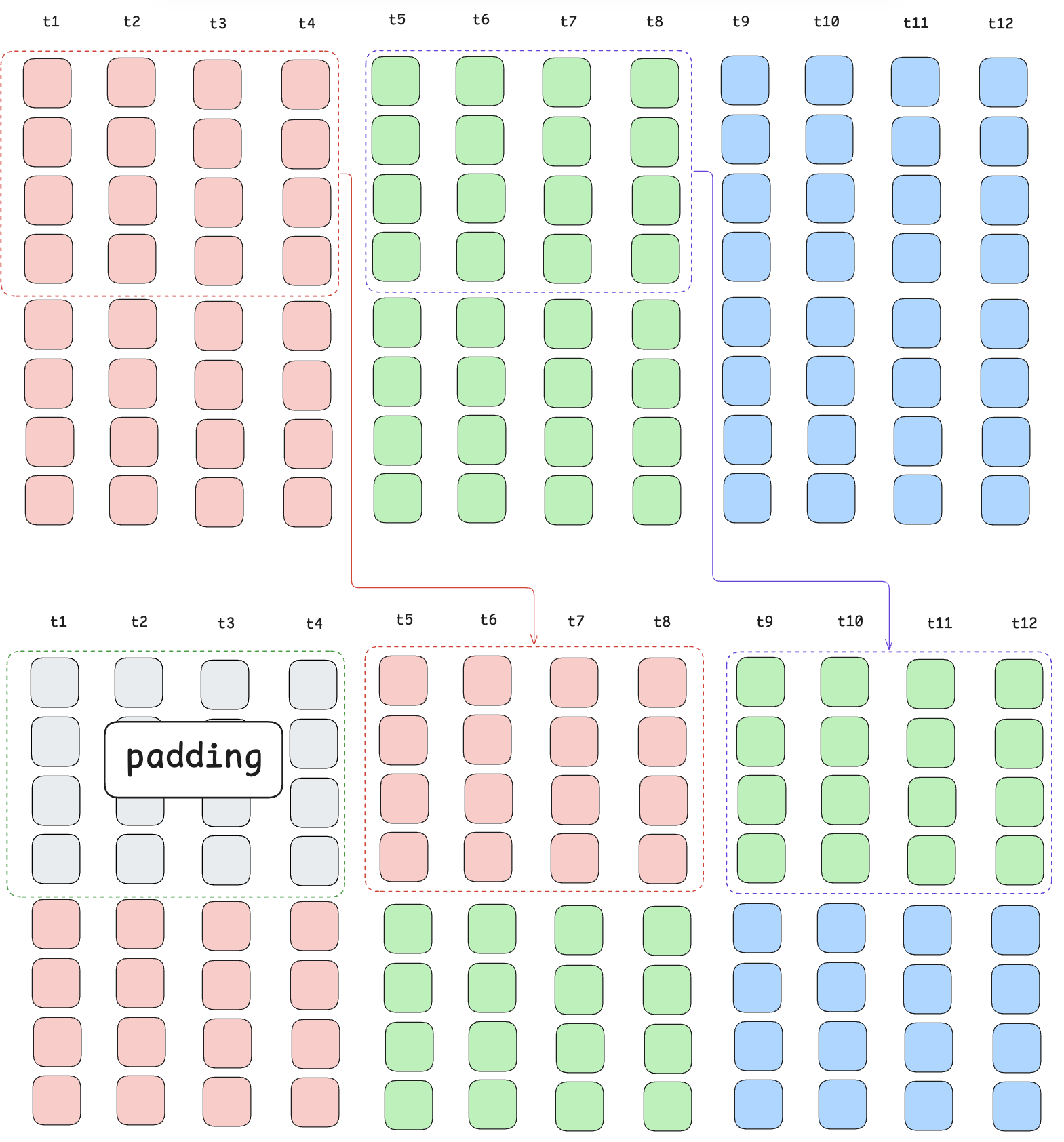
$[t1,t2,t3,t4]$ is group1, $[t5,t6,t7,t8]$ is group2, and the upper half of group1, $d$, is shifted into the upper half of group2. Since the upper half of group1 has been shifted away, all of its values need to be set to $-INF$. In PyTorch this can be written as:
 1def overlap_transform(x: torch.Tensor, pad_value=0.0) -> torch.Tensor:
 2    # x: [B, G, m, 2*d], m=4
 3    B, G, m, two_d = x.shape
 4    d = two_d // 2
 5    out = x.new_full((B, G, 2 * m, d), pad_value)
 6
 7	# up d-dimension
 8    out[:, :, m:, :] = x[:, :, :, d:]
 9
10	# down d-dimension
11    out[:, 1:, :m, :] = x[:, :-1, :, :d]
12
13    return out
14
15# KV Path Overlap
16kv_overlap = overlap_transform(kv, pad_value=0.0)
17# Gate Path Overlap
18logits_overlap = overlap_transform(
19    gate_logits + ape,
20    pad_value=float("-inf"),
21)
In the HCA/CSA structures there are two different 11 here:
- HCA’s KVCompressor uses m=128 and does no overlap. It compresses to the extreme and ignores the relationship between adjacent segments.
- CSA’s KVCompressor uses m=4 and does overlap. It compresses more coarsely but pays much more attention to detail.
3.2 Locality: Combining Sliding Window Attention with Sparse Attention
When a person reads, our brain is more familiar with the letters/words it has just finished reading, and has only a rough impression (compressed information) of things far in the past. DeepSeek’s CSA builds a similar mechanism: it uses a sliding window to apply full, uncompressed attention to the most recent 128 tokens, while for content before those 128 tokens it uses the KVCompressor + SparseAttention approach described above to compress and selectively attend. The comparison with DSA is shown below:
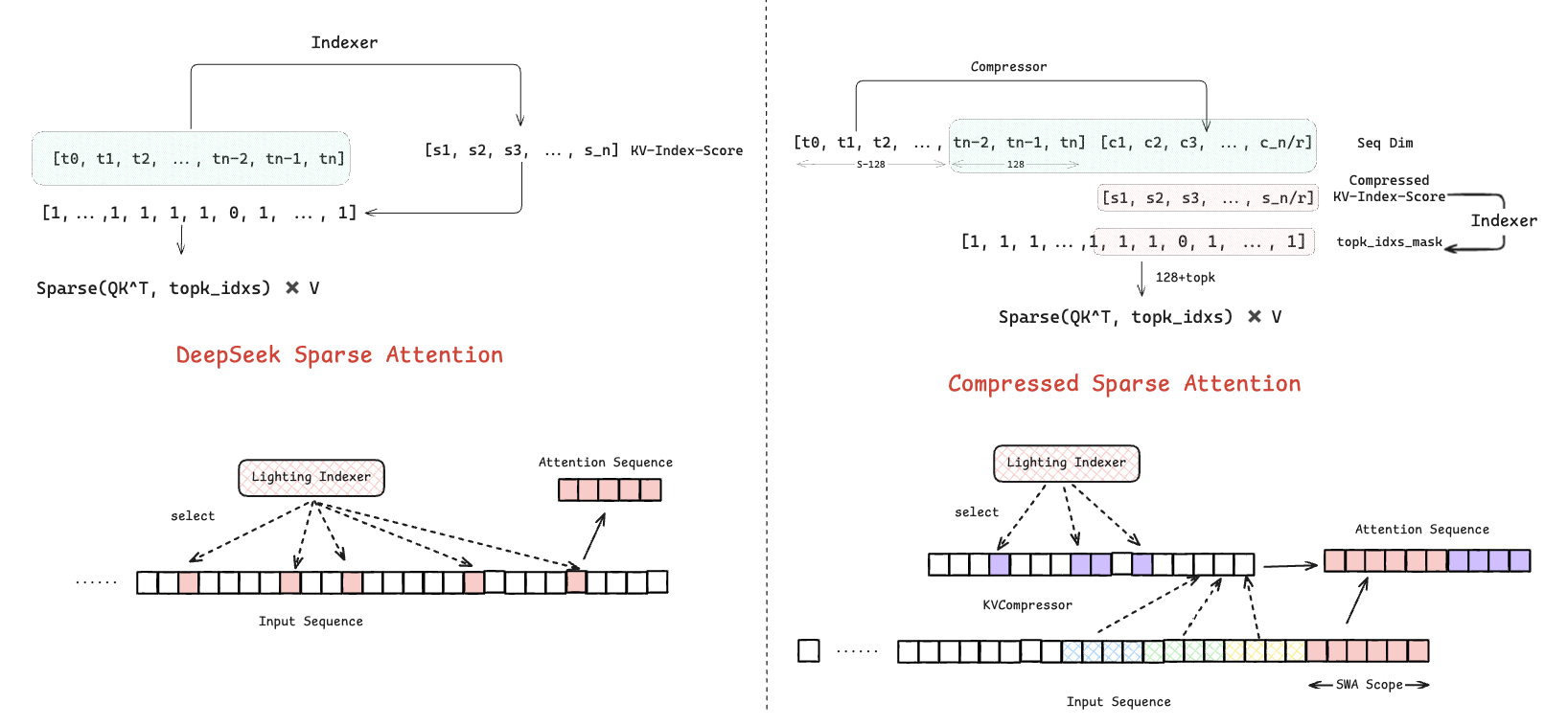
In DSA, DeepSeek uses an Indexer to compute the topk(2048) tokens most relevant to the current information, whereas in V4’s CSA structure:
- First, the 128 tokens are fully included in the final attention sequence to be computed.
- The $S-128$ tokens are compressed using KVCompressor.
- An indexer is used on the compressed tokens to select the most relevant topk information.
- Based on the 128 trailing tokens and the compressed token indices produced by the Indexer, an overall mask is finally generated and fed into Sparse Attention to complete the computation.
This approach accounts for both nearby information and long-range compressed information. More importantly, thanks to KVCompressor we only need to cache the KV of the most recent 128 tokens plus the KV compressed by KVCompressor, which greatly reduces the storage pressure of the KV cache. I made a simple table here to compare the KV cache gap (ignoring the local window, compression state, and quantization metadata overhead).
| Architecture | Main attention cache | Indexer cache | Total elements/token | Relative to MLA |
|---|---|---|---|---|
| Original MLA | 512+64=576 | 0 | 576 | 100% |
| V3.2’s DSA | 512+64=576 | 128 | 704 | 122.2% |
| V4’s CSA, m=4 | 512/4=128 | 128/4=32 | 160 | 27.8% |
Insight | CSA solves both complexity and KV cache
As you can see, compared with MLA and DSA, CSA both solves MLA’s computational complexity problem for long-range computation and compresses KV cache usage to about 1/4 of what it was.
3.3 State Cache: The short-lived state that must be kept during Decode
Besides the long-range KVCache, the CSA structure in V4 also introduces a StateCache. The State Cache is the small piece of state the model needs to keep and continuously update in order to process the next token. In V4, it mainly consists of the KV of the local window, plus the intermediate state the compressor still needs to use. It splits into two parts:
- Sliding Window KV: because the Sliding Window is constantly updated during computation (constant space), and there is no need to save historical state
- KV-Compressor state: following the
m=4、overlap=Truefrom just now:
Previous group: token 0, 1, 2, 3
Current group: token 4, 5, still missing 6, 7
At this point the compressor needs to keep:
- The projection results and gate logits of the current incomplete group, to be computed together once 6 and 7 arrive.
- The representation and gate logits of the previous group used for overlap, because the next compressed KV needs to aggregate information from the previous group and the current group.
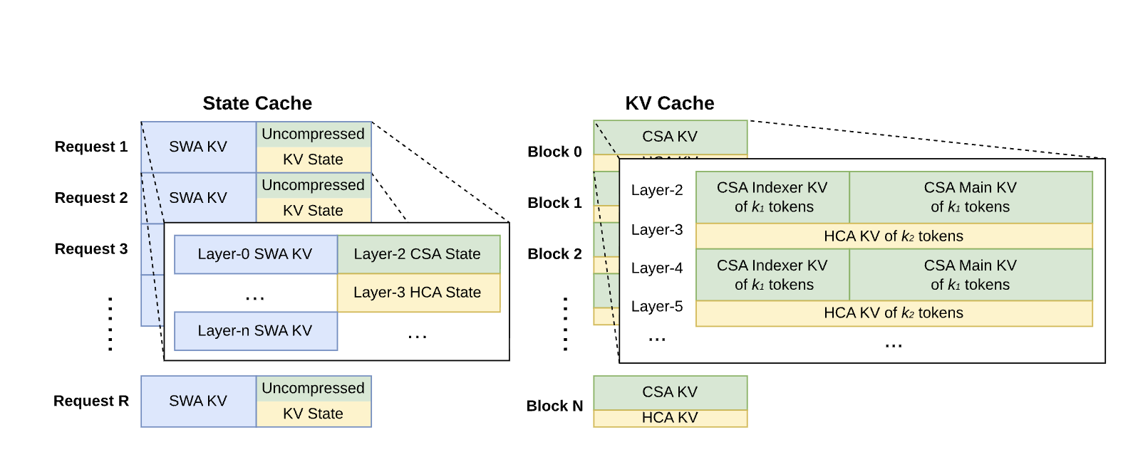
We can analyze the two Caches like this:
| Cache | What it stores | Does it grow with history length? |
|---|---|---|
| Historical compressed cache | The already-generated compressed KV and the corresponding Indexer Key | Yes |
| State Cache | The KV of the most recent window, the working state of the compressor | Fixed capacity per request, per layer |
Insight | Where State Cache fits
State Cache is mainly the short-lived state introduced during computation; there is no need to save the per-token KV of the entire history.
3.4 Heavily Compressed Attention: Extreme Compression + MQA
HCA is a relatively very simple structure. Like CSA, it combines sliding window attention with a Compressor structure. The sliding window uses a window of 128 tokens, and the Compressor performs extreme compression directly (128 tokens compressed into 1 token), then after concatenation it directly does MQA.
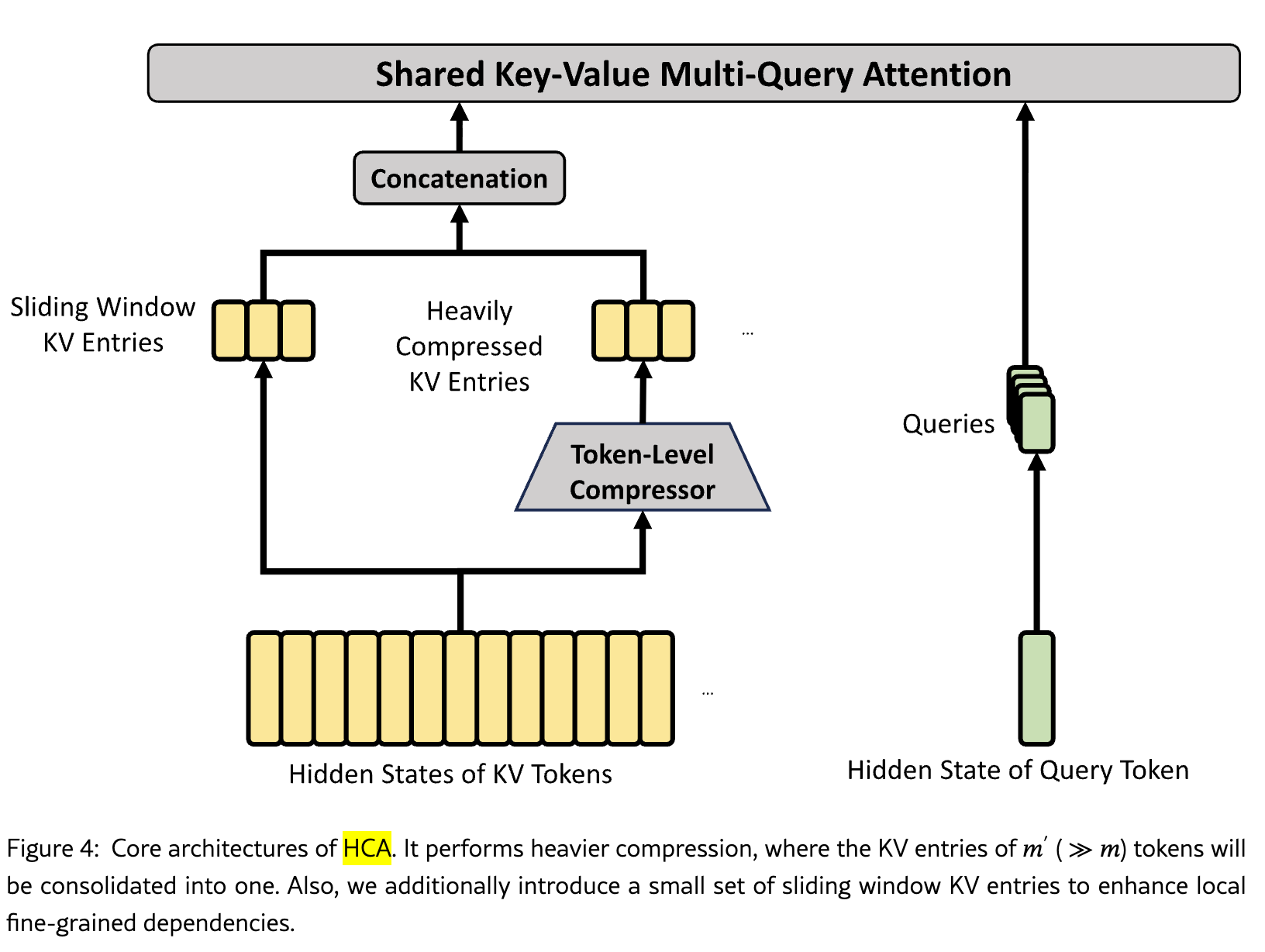
3.5 Stacking CSA and HCA: the overall organization of V4
In its overall structure, DeepSeekV4 is organized by stacking HCA and CSA, and V4Pro and V4Flash use different stacking schemes:
- V4Pro starts with two HCA layers, followed by CSA+HCA stacked at 1:1
- V4Flash starts with SWA, followed by CSA+HCA stacked at 1:1
4. CSA2: More Extreme Compression and Sharing
From the discussion above, we can see that CSA mainly compresses the KVCache along the sequence dimension, merging the information of multiple tokens into a single entry. But looking at the model as a whole, each layer still needs to maintain its own cache. Even if a single layer compresses well, once you multiply that by dozens of layers, the overall storage pressure is still considerable.
The IndexCache introduced earlier already showed that the key positions selected by adjacent layers are similar, so the Top-K results can be reused. CSA2 pushes further in this direction, bringing the KV of the main attention, the K of the Indexer, and the Top-K indices all into the scope of cross-layer reuse. At the same time, combined with CED, the Decoder’s global KV is generated from the Encoder’s output, further reducing the processing overhead of long inputs.
4.1 Simplifying the Compressor: Removing Overlap and Sharing the Compression Result
First, the Compressor. CSA2 still uses Gate Pooling to aggregate m consecutive tokens into a single KV entry, but it drops the original Overlap Transform and the APE inside the compressor. As a result, the span involved in one compression shrinks from 2m tokens spanning two groups to the m tokens of the current group12.
Note | Dimension comparison with CSA
The Overlap Transform expands the dimension of $[B,G,4,2d]$ to $[B,G,8,d]$, so it can be thought of as compressing 2m tokens. CSA no longer maps $X$ to a $2d$ dimension, but maps it directly to $d$, skipping the overlap step in the dimension
Using the notation from earlier and ignoring the trailing incomplete group, this can be written as the following pseudocode:
1# x: [B, S, d_model], simplified here so S is divisible by m
2kv = kv_proj(x).reshape(B, S // m, m, d)
3gate = gate_proj(x).reshape(B, S // m, m, d)
4
5# Compute the weights of m tokens within each group separately for each channel
6weight = gate.softmax(dim=2)
7compressed_kv = kv_norm((kv * weight).sum(dim=2))
8# compressed_kv: [B, S // m, d]
Another change is in the Indexer: CSA2 projects the Indexer K directly from the compressed representation before RoPE is applied, eliminating the separate Indexer compression path. After that, the main KV and the Indexer K each undergo positional encoding and quantization separately. In other words, the KV and the Indexer share a single Compressor. The overall result is shown in the figure:
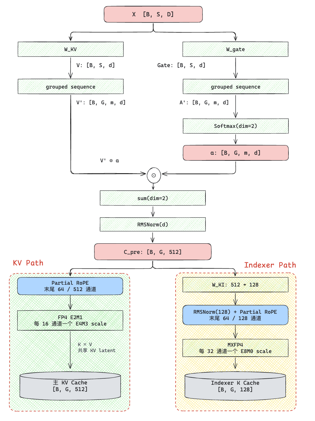
4.2 The overall flow of CSA2: local window + global retrieval
Plugging the Compressor back into the backbone, CSA2 still keeps the basic idea of CSA introduced earlier:
- Each layer maintains a local window KV of the most recent 128 tokens.
- The Indexer selects at most 512 entries from the causally visible global KV.
- The main Query attends to both the selected global entries and the local window, producing this layer’s attention output.
Below is the Full Mode that executes the complete computation flow. The dimensions in the figure use the actual configuration of V4.1-Flash: the main Query has 64 heads, each 512-dimensional; the Indexer has 32 query heads, each 128-dimensional. As shown in the figure:
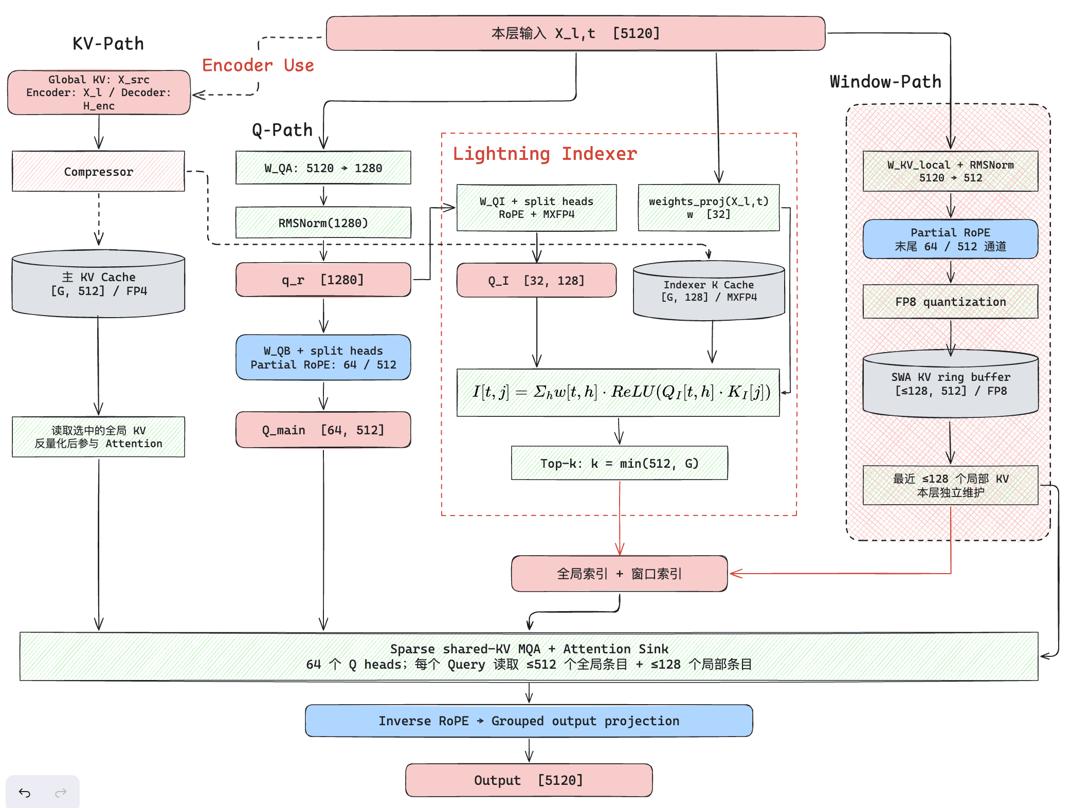
The overall path has four parts:
- KV-Path: directly obtains the compressed KV sequence. During attention, it is masked by the mask produced by the indexer. The KV output has two possibilities:
- In the Encoder part, directly use this layer’s input
- In the Decoder part, directly use $H_{enc}$, i.e. the Encoder’s output.
- Indexer: this part, like CSA and DSA, is used to find the topk tokens most relevant to the current compressed KV. Unlike CSA, where the Indexer’s K is computed by a separate Compressor, in CSA2 the Index K directly shares the output of the KV Compressor.
- Q-Path: computes the Query information.
- Window-Path: this part is used to produce the window information for the most recent 128 tokens.
4.3 From IndexCache to KVCache: Three Cross-Layer Sharing Modes
The IndexCache above mainly reuses the result of “which positions to look at”, while CSA2 goes further and shares “the content at those positions” as well.
To keep sharing reasonably flexible, CSA2 statically configures each layer into one of three modes:
| Mode | Global main KV and Indexer K | Top-K index |
|---|---|---|
| Full | Generated by this layer | Recomputed by this layer |
| Reindex | Reuses the cache of an earlier Full layer | Recomputed with this layer’s Indexer Query |
| Reuse | Reuses the cache of an earlier Full layer | Reuses the latest index produced for that cache |
The paper has a figure that illustrates these three modes nicely.
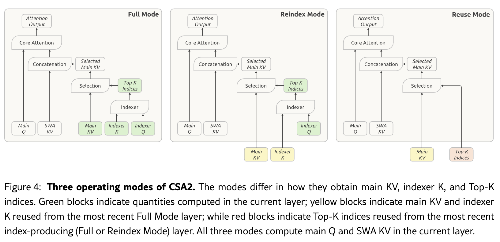
You can think of it as several people sharing one set of materials: someone re-highlights the key points, someone else follows the positions marked by the previous person, but each person still interprets the content according to their own question. Mapped onto the model, all three modes keep this layer’s own main Query, local-window KV, and attention weight computation. So even after sharing the cache and the index, each layer can still produce a different output. What Reuse saves is the Indexer’s Query, scoring, and Top-K — it does not skip the main attention.
Note | What does Full Mode mean
Full Mode here means running the complete CSA2 computation flow; the main attention is still sparse. Sharing also happens across different layers at the same token position; when generating the next token, retrieval is redone based on the new Query.
4.4 Hierarchical Indexer: narrowing the search range of later layers
Cross-layer reuse reduces the number of Indexer inference passes, but the Reindex layers that remain may still face very long history sequences. Even if we only select 512 entries, finding those 512 positions requires first scoring the candidate positions. To this end, V4.1-Flash introduces a Hierarchical Sparse Indexer in the Decoder, 13 letting the later Reindex layers continue searching within the candidate range filtered out by the earlier layers. Because of the CED discussed later, this HSI structure is used only in the Encoder process. The overall structure is shown in the figure below:
The concrete process can be divided into two steps:
- The first layer performs a full-range retrieval. It scores all causally visible positions and selects the Top-512 used by this layer’s attention; at the same time, every 8 positions form a block, the highest score within the block is taken as the block score, and at most 2048 blocks are selected, forming a candidate pool of at most 2048×8=16384 positions. The implementation also ensures that the most recent visible block is retained.
- Subsequent Reindex layers re-score within the candidate pool. Each layer uses its own Indexer Query to select its own Top-512 from these candidate positions. The later Reuse layers continue to reuse the latest index.
Two quantities need to be kept distinct here: 16384 determines the search range of the subsequent Indexers, while 512 determines how many global entries the main attention reads.
The first round still has to scan the full visible history, so it still carries a cost that grows with context length. What the figure describes is the hierarchical retrieval algorithm; making the subsequent computation actually scale with the candidate pool size requires a corresponding sparse kernel. The official minimal Python implementation computes the full scores first and then applies a candidate mask14.
4.5 CED: Generating the Decoder’s Global KV Ahead of Time
Beyond compression and shared caches, V4.1-Flash also reduces Prefill computation for long inputs through a Causal Encoder-Decoder, or CED. You could call it a return to first principles — the overall structure is actually similar to the original Transformer.
It splits the 40-layer backbone into a 20-layer Causal Encoder and a 20-layer Decoder. The global KV the Decoder needs is obtained by projecting from the Encoder’s final hidden state $H_{enc}$. This way, when processing historical input, the global cache the Decoder will read is ready as soon as the Encoder computation finishes.
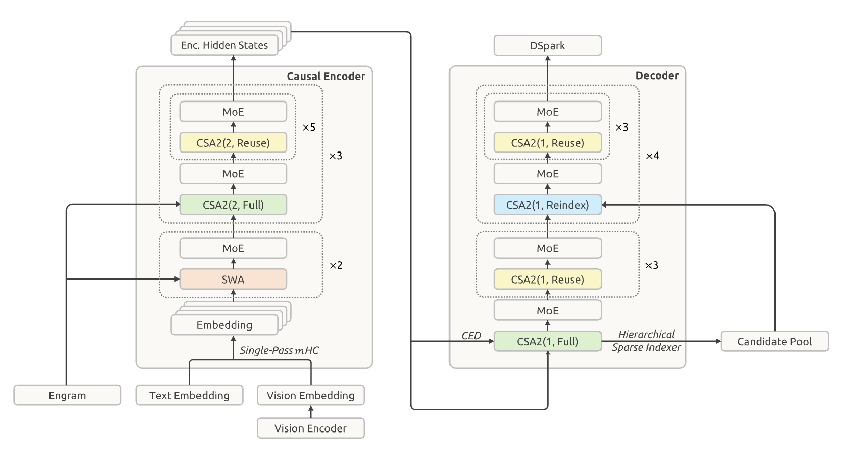
However, the Decoder’s local window KV still depends on layer-by-layer computation. To handle this, deployment uses SWA Bounded Replay to redo the Decoder computation for the last 128 tokens of the prompt, approximately restoring the required window state.
Important | Different from the original Transformer
The order of computation in CED: Prefill computes only the Encoder; Decode computes Encoder+Decoder. This differs from the original Transformer, where after the Encoder computation, producing subsequent tokens only requires running the Decoder.
Insight | What CED saves is the Prefill over historical input
So for a long prompt, most positions only need the full Encoder computation, and the Decoder mainly redoes the tail window; once in Decode, every new token still passes through all 40 layers. What is saved here is mainly the Prefill cost over historical input.
4.6 CSA2 Summary
CSA2 makes substantial improvements over CSA — DeepSeekV4.1-Flash is already hugely different from the overall DeepSeekV4 architecture. To sum up, DeepSeekV4.1-Flash + CSA2 mainly upgrades in these areas:
- Simplified Compressor, shared compression output: The Compressor is reworked to drop Overlap and APE, and a single KVCompressor can now produce the downstream features for both the Indexer and the KV.
- Three levels of sharing: this minimizes the overhead introduced by Indexer computation as much as possible.
- Hierarchical Sparse Indexer: the Decoder’s first Full layer scans the visible history and, beyond selecting this layer’s Top-K, also builds a larger candidate pool via block-level filtering. Subsequent Reindex layers pick their own Top-K from this candidate pool, reducing repeated full-range retrieval. The candidate pool can be shared, but the positions each layer ultimately attends to can still differ.
- Introducing CED to lower the prefill cost of long inputs: the Decoder’s global KV is generated directly from the Encoder’s final output, so most prompt tokens only need the Encoder computation, plus a supplementary Decoder computation over the trailing window. During decode, each new token still goes through the full Encoder and Decoder.
- Introducing FP4 KV15: this is mainly an engineering optimization — the global main KV uses FP4, the Indexer K uses MXFP4, and combined with cross-layer sharing this brings the whole model’s global cache footprint down to about 890 bytes/token, roughly a quarter of V4-Flash.
5. Summary
From MLA to DSA to CSA and CSA2, DeepSeek has consistently pursued the tradeoff between algorithms and engineering. While satisfying the algorithm’s requirements, it has already drastically reduced the GPU memory and memory bandwidth demands of the KVCache, as well as the compute demands of Prefill/Decode. It even made a radical architectural change like CED in DeepSeekV4.1-Flash — all I can say is that the entire algorithm team and engineering team have real strength and boldness. I also really enjoy using DeepSeekV4.1-Flash; thanks to DeepSeek’s engineering optimizations, it can basically sustain 200-400TPS over the long run. Although the RL of DeepSeekV4.1-Flash still needs continuous tuning and improvement, its formidable engineering capability truly pushes the Agent experience to the extreme.
Because DSA’s Indexer only needs to produce scores suitable for Top-k selection, and ReLU plus per-head weighting is a computationally cheap way to do multi-head scoring. The paper notes: ReLU was chosen for throughput reasons ↩︎
When training the Indexer, Softmax is still used: the paper applies Softmax to the final $I$, then aligns it with the main attention distribution via KL divergence, so the Indexer learns which tokens are worth keeping. At inference time only Top-k is taken; once selected, the main MLA computes its own attention scores and Softmax weights. ↩︎
Temporal Correlation Meets Sparse Attention: Guess-Verify-Refine Top-K for Blackwell ↩︎
DeepSeek: DeepSelect The kernel DeepSeek open-sourced alongside DeepSeekV4.1-Flash ↩︎
FlashMLA Blog: A Deep Dive Into The Flash MLA FP8 Decoding Kernel on Hopper: With a smaller topk, the relative overhead of the kernel’s prologue and epilogue becomes larger compared with dense decoding with long context length. If we set topk to a larger value, such as 32768, this kernel can achieve up to 460 TFLOPS ↩︎
Implementations that skip the Indexer under short context vLLM (the corresponding parameter is
enable_short_prefill_scoring_skip) SGLANG (the corresponding environment variable isSGLANG_DSA_PREFILL_DENSE_ATTN_KV_LEN_THRESHOLD) ↩︎MiniMax Sparse Attention: https://arxiv.org/pdf/2606.13392 ↩︎
IndexCache: https://github.com/THUDM/IndexCache ↩︎
Heterogeneous KV Entries in DeepSeek-V4: https://arxiv.org/html/2606.19348#S3.SS5.SSS1 ↩︎
A simple Hierarchical Sparse Indexer implemented officially in Pytorch https://huggingface.co/deepseek-ai/DeepSeek-V4.1-Flash/blob/main/inference/model.py#L583 ↩︎
DeepSeekV4.1-Flash Paper section 6: In this work, we introduce DeepSeek-V4.1-Flash, a multimodal Mixture-of-Experts (MoE) model with support for contexts of up to one million tokens. Through joint optimization of model architecture, cache precision, and deployment strategy, DeepSeek-V4.1-Flash pushes the limits of KV cache compression. Its Causal Encoder-Decoder (CED) architecture enables the model to activate only 8B parameters per token during prefill, compared with 16B during decode, improving cost efficiency for input-heavy agentic workloads. At equal sequence lengths, cross-layer KV cache reuse in Compressed Sparse Attention 2 (CSA2) and FP4 KV caching reduce its global KV cache footprint (always in HBM) to 890 bytes per token, roughly 1/4 of the corresponding footprint of DeepSeek-V4-Flash. SWA Bounded Replay further reduces its persistent KV cache footprint (always on SSD or in host memory) to roughly 1/8 of that of DeepSeek-V4-Flash. These reductions alleviate HBM and SSD capacity pressure while the model delivers substantially better overall performance than DeepSeek-V4-Flash. Despite possessing a significantly smaller parameter footprint than contemporary open-source models such as GLM-5.3 and Kimi-K3, DeepSeek-V4.1 achieves comparable—and in several tasks, superior—performance across key benchmarks. ↩︎