DeepSeek's attention evolution - [MLA]
Foreword: After reading the DeepSeekV4.1 paper and seeing that DeepSeek had once again made major changes to the model architecture, I was quite excited. So I looked back at DeepSeek’s incremental improvements to the model architecture and wrote this series of articles in the gaps while waiting for agents to finish running and slacking off at work — a summary of what I’ve learned about model architectures over the year since I moved into AI Infra.
This article mainly covers the changes to the attention architecture over the course of DeepSeek’s model evolution, and also shows how DeepSeek’s architecture evolved step by step from the perspective of KV cache optimization — in particular, it gives a fairly detailed account of the algorithmic and engineering tradeoffs in the architecture. DeepSeek’s attention choices and design really are excellent, with something uniquely insightful from both the engineering and algorithmic angles, so much so that the later domestic large models — the GLM5.x / Minimax3.x / Kimi2.x series — all adopted DeepSeek’s design or made some improvements on top of it.
1. MHA for sequence modeling, the birth of the Transformer
1.1 Background and Problem
This is a classic problem. The MultiHead Self-Attention structure was born alongside the Transformer, mainly to replace RNN/LSTM (Recurrent Neural Network) and solve two problems in sequence modeling.
- Long-range dependency modeling (the core problem): RNN/LSTM always use a fixed state $S$ to compress all past state information, so when the input sequence is long, excessive compression causes long-range information to be lost.
- Parallelism (a computational efficiency problem): RNN/LSTM can only compute serially. As shown below, when an RNN computes a state it must do so serially, only after $S_{t-1}$ has finished computing. Attention can be computed in parallel — a single matrix/tensor can compute all positions at once.
The figure below 1 makes these two problems immediately clear.
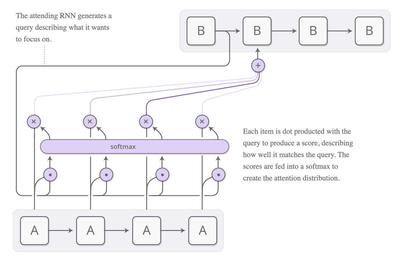
When an RNN computes the next token, its computation over the preceding sequence is serial: it finishes computing the previous piece of information, stores the state, and only then computes the next piece of information.
1.2 Introducing Attention - token2token modeling of sequences
To solve these two problems, Transformers introduced Attention at design time to model sequences. Its structure is shown in Figure 1: it directly performs Pair2Pair computation over the entire sequence, thus solving the previous two problems. In practice, though, it is a bit more abstract — it turns the sequence Pair problem into a lookup problem.
- Map the input $X$ to two vectors $K$ and $V$, where, just like in a computer, KV is a pair.
- Map $X$ to an $Q$; this $Q$ is what we usually call the query vector.
- Compute the relationships between the tokens of $X$ by computing relevance via $score=softmax(QK^T)$.
- Finally multiply by the $V$ vectors and do a weighted sum, $O=score \cdot V$. Of course, Transformers also handles some details — for example, to deal with $QK^T$ blowing up as the dimension $d$ grows, which pushes $softmax$ into the saturated gradient region, it applies a simple Scaled Dot-Product Attention, changing the score to $score=softmax(\frac{QK^T}{\sqrt{d}})$.
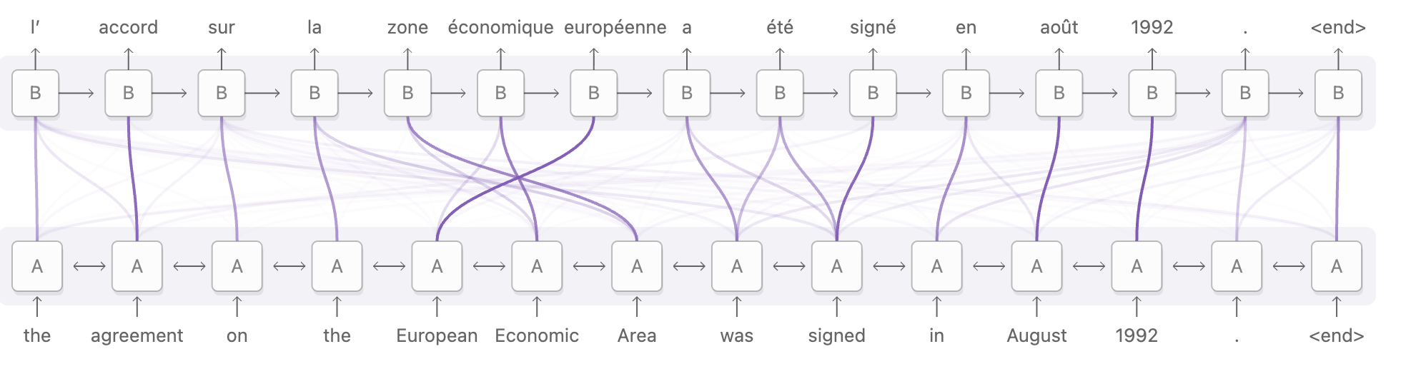
Now let’s look at how these two problems are solved:
- Why it solves the long-range dependency problem: Attention directly computes the relationship between tokens at any two positions, so there is no problem of state being accumulated and overlapped all along.
- Why it solves the computational efficiency problem: as in 1, because it can be abstracted as an $O=score \cdot V$, which is just a multiplication of two matrices, so the GPU can compute it very efficiently.
1.3 MultiHead: mapping multi-dimensional information
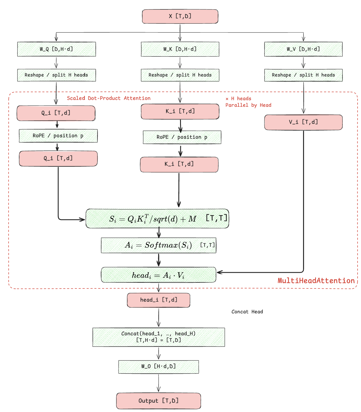
At the same time, to better represent multi-dimensional information, Transformers introduced the MultiHead structure. That is, when computing, the input $X$ is first mapped into multiple heads, in order to aggregate more kinds of information. The original text describes it as 2:
Multi-head attention allows the model to jointly attend to information from different representation subspaces at different positions.
So the final MHA becomes this structure:
$$\text{MultiHead}(Q, K, V) = \text{Concat}(\text{head}_1, \dots, \text{head}_h)\\, W^O$$where each head is:
$$\text{head}_i = \text{Attention}(Q W_i^Q,\ K W_i^K,\ V W_i^V)$$The attention of each head is:
$$\text{Attention}(Q,K,V) = \text{softmax}\\!\left(\frac{QK^T}{\sqrt{d_k}}\right)V$$The overall structure is shown in the figure below
1.4 The problem with MHA: bloated compute and storage
So we’ve covered all the benefits of MHA — but what’s the cost of modeling things this way?
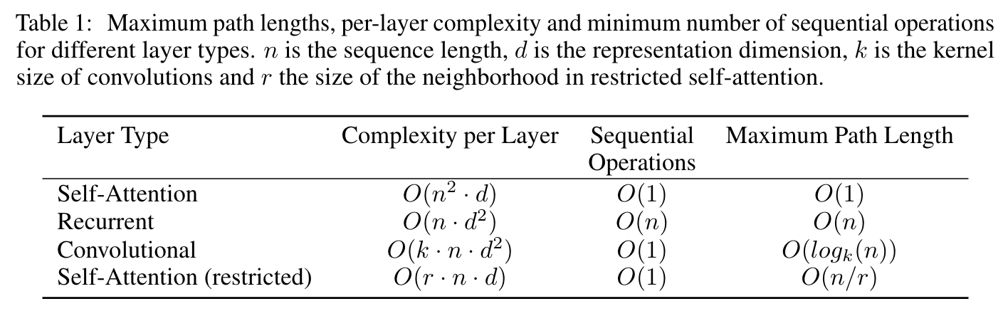
The Transformers paper has a table laying out that cost: because of the Pair2Pair modeling, the computational complexity becomes $O(N^2)$, and the intermediate KV storage grows linearly with sequence length N. By comparison, an RNN has time complexity $O(N)$ and space complexity $O(1)$. So once large models arrived and long-sequence problems showed up, people started deriving LinearAttention (which you can think of as an RNN variant) / SWA to reduce the computational complexity of attention and the space taken up by the KV cache under long sequences.
1.5 GQA/MQA - KV reuse
Let’s set aside SWA and LinearAttention, the two structures that see a lot of use these days, and first look at the most frequently discussed evolution: MHA/GQA/MQA.
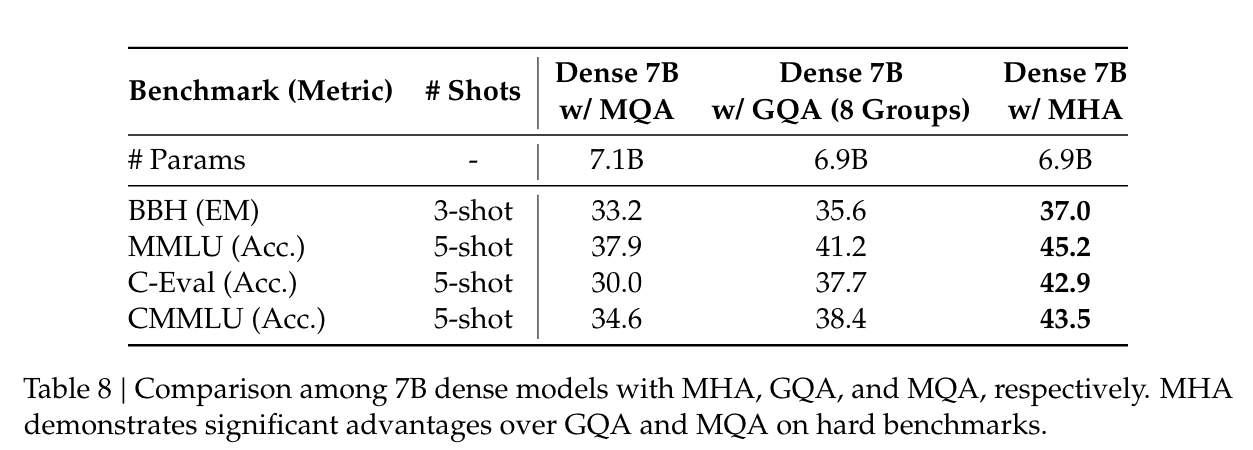
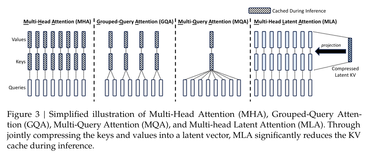
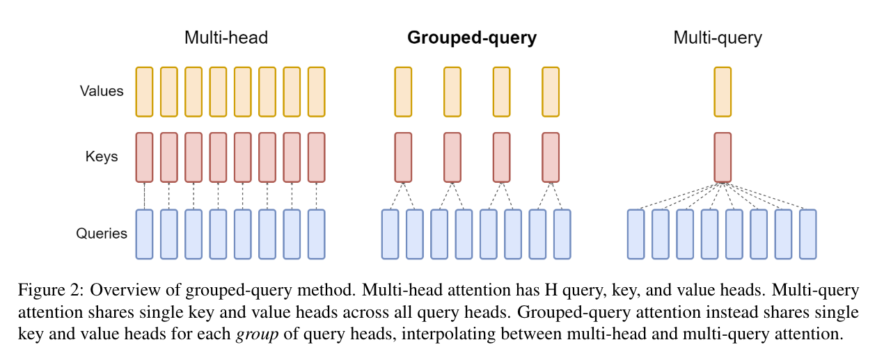 Here we can bring out that diagram everyone has seen countless times, from 3. Both approaches reduce compute and KV cache storage by having multiple heads share the KV. GQA has G heads sharing one set of KV, while MQA has all heads sharing all the KV, but MHA still delivers better results by comparison. For example, the early Qwen2/Llama/GPT-OSS series used GQA.
2. Compressing the KV into a Latent - From MHA to MLA
2.1 The Problem and Background
Here we go again with the same old topic. From the perspective of LLM inference engineering, for an LLM with a Decode-Only architecture, the inference process can be split into Prefill and Decode. Prefill focuses on computing the KV cache of the preceding sequence and the first token, while Decode iteratively computes the subsequent tokens. Prefill is compute-bound, whereas Decode is memory-bandwidth bound. Since from an overall engineering standpoint memory-bandwidth bound is the harder problem to solve, the emergence of MLA is aimed squarely at addressing the memory-bandwidth bound problem of the KV cache during inference.
2.2 LoRA: Down-projection and Up-projection
How do we solve this? The idea is actually quite simple: use LoRA, which is commonly used in DL, to do a down-projection, then compute attention, and after the computation is done, map back to a high dimension through a matrix for output. This trick is widely used in various neural network structures in deep learning. The recent Latent-MoE follows the same idea, except it turns MHA into MoE, reducing the communication volume of MoE through dimensionality reduction.
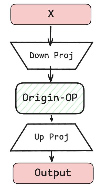
What is LoRA: It exploits the fact that high-dimensional data matrices contain a large amount of redundancy and that the effective information is concentrated in only a few principal directions. It represents the original $d \times k$ data with a rank $r$ that is far smaller than it (first compressing to an $r$-dimensional bottleneck, then up-projecting back), reducing the data volume from $d\times k$ to $r\times(d+k)$, thereby greatly lowering computation and GPU memory (e.g., compressing the KV cache) while keeping information loss controllable. In short, it uses a lower-dimensional vector with higher information density to represent a high-dimensional vector, thereby reducing storage/computation complexity.
On this idea, MLA makes some modifications to MHA. The core operation is mainly to reduce the amount of KV cache during computation, so we can see that MLA computes Q/K by directly doing a matrix multiplication with a down-projection matrix, reducing the previous dimension to a low-rank representation $C$. For this point, the structure can be obtained by changing the previous MHA into an MHA with LoRA, as shown in the figure: 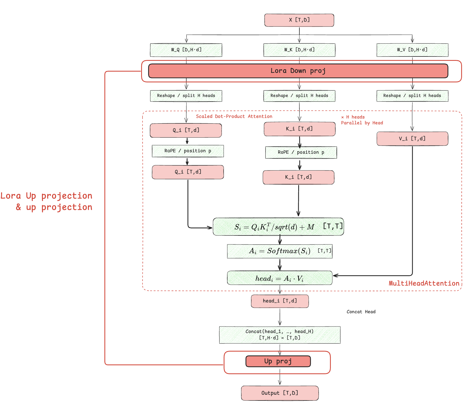
But for inference performance, a small structural change was introduced: splitting RoPE out of the main K computation path, with a separate branch to compute the RoPE of $K$. Why is this? Before explaining the principle, let me first introduce a trick commonly used in inference, namely matrix absorption, which is also a very simple mathematical technique.
2.3 Matrix Absorption
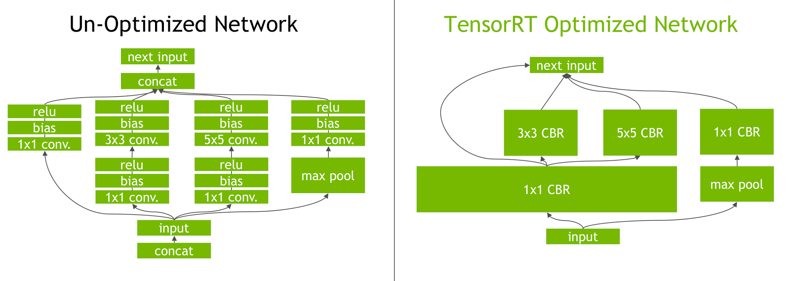
In model inference, many structures can be merged mathematically. For example, back in the CNN era, TensorRT often performed this kind of optimization, as shown in the figure below 4, merging multiple operations into a single operation. This behavior is also commonly used in inference optimization in the LLM era. For instance, in the figure above, when computing QKV, we can actually merge the three mapping matrices in $Q=W_qX$, $K=W_kX$, $V=W_vX$ into a single $[Q,K,V] = [W_q, W_k, W_v]X$. That way we can use one kernel to compute all three outputs at once, greatly simplifying kernel launch and setup work.
Going further, some operations require passing through two mappings at once, for example
$$O = W_b(W_aX)$$We can also transform this via the associativity of matrix multiplication into
$$O = (W_bW_a)X = W_{fuse}X$$At model load time, we precompute $W_{fuse}$ in advance, so that during inference we don’t need to perform multiple computation operations. This operation has a dedicated name: Matrix Absorption. Its benefits are obvious — it accelerates inference. But it also has a downside: it loses precision5.
2.4 The RoPE branch: the positional encoding problem and its solution
Back in MLA, in DeepSeek’s paper the authors also wanted to optimize MLA inference through Matrix Absorption: even if accuracy drops slightly, it buys an overall speedup in inference. That’s when RoPE turns out to be the stumbling block. Compressing directly with low-rank hits a pitfall: RoPE is position-sensitive.
- If you apply RoPE to the $k^C$ recovered from the compressed representation, then $W^{UK}$ becomes coupled with the “RoPE matrix tied to the current token position”;
- Because matrix multiplication is not associative, $W^{UK}$ cannot be absorbed into $W^Q$, and at inference time you have to recompute K for every prefix token → the cache was compressed for nothing. Algebraically it can still be merged, but you lose the optimization MLA needs: “transform the current Q once and reuse it for all historical positions.”
Let’s treat the current $q$ as having already had its own RoPE applied, and look only at the historical K side.
Without RoPE, all historical Keys use the same matrix $U$:
$$k_1=Uc_1,\qquad k_2=Uc_2,\qquad k_3=Uc_3$$So you only need to compute one $\widetilde q=U^\top q$ and dot it with each $c_1,c_2,c_3$.
With RoPE, each position has an extra, different rotation matrix:
$$k_1=R_1Uc_1,\qquad k_2=R_2Uc_2,\qquad k_3=R_3Uc_3$$Move these transforms over to the Q side and it becomes:
| Which historical position it’s compared against | The transformed Query required |
|---|---|
| Position 1 | $\widetilde q_1=U^\top R_1^\top q$ |
| Position 2 | $\widetilde q_2=U^\top R_2^\top q$ |
| Position 3 | $\widetilde q_3=U^\top R_3^\top q$ |
Now you need three different $\widetilde q$. With ten thousand historical positions, you might need ten thousand.
Even if you pre-merge $R_jU$ into a matrix $M_j$, it’s still a different $M_j$ per position, each of which has to be applied separately to the current Query.
So how do we solve this? Spin off a dedicated branch to compute RoPE, and at the same time convert the earlier $X+RoPE$ approach into the $[X;RoPE]$ approach, so that the parts without RoPE can keep enjoying the nice matrix absorption trick. But if K changes like this, Q has to change the same way. So MLA becomes this structure:
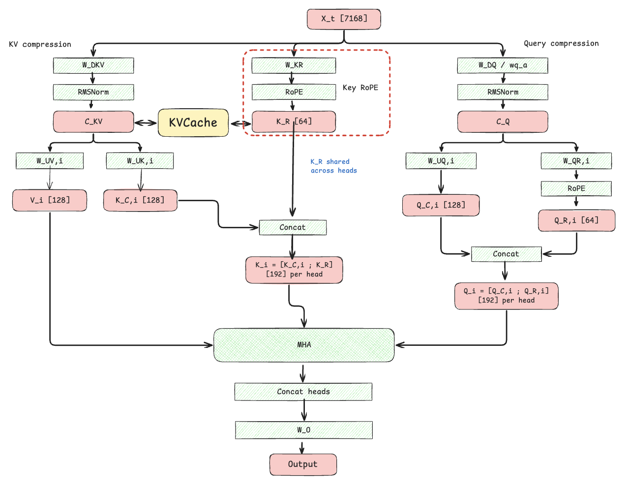
A structure that is compatible both engineering-wise and algorithm-wise. The DeepSeekV2 paper also ran ablations: MLA is strictly better than MQA and GQA in quality.
 To sum up how it differs from MQA and GQA, one figure from the DeepSeekV2 paper is worth a thousand words
2.5 MQA/MHA Dual Form
Following matrix absorption, can we optimize inference further? At this point we could actually go one step further with Absorption and merge all subsequent parameters. The answer is yes — we can even fully convert MLA into MQA form. The DeepSeekV3.2 paper appendix also mentions this optimization:
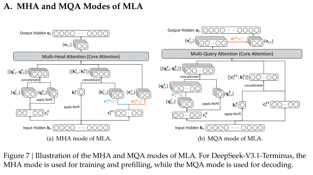
How is it done? It’s actually based on some very simple mathematical merge operations. Here I’ll just summarize Su Shen’s derivation6. If you’re interested, you can read Su Shen’s derivation directly:
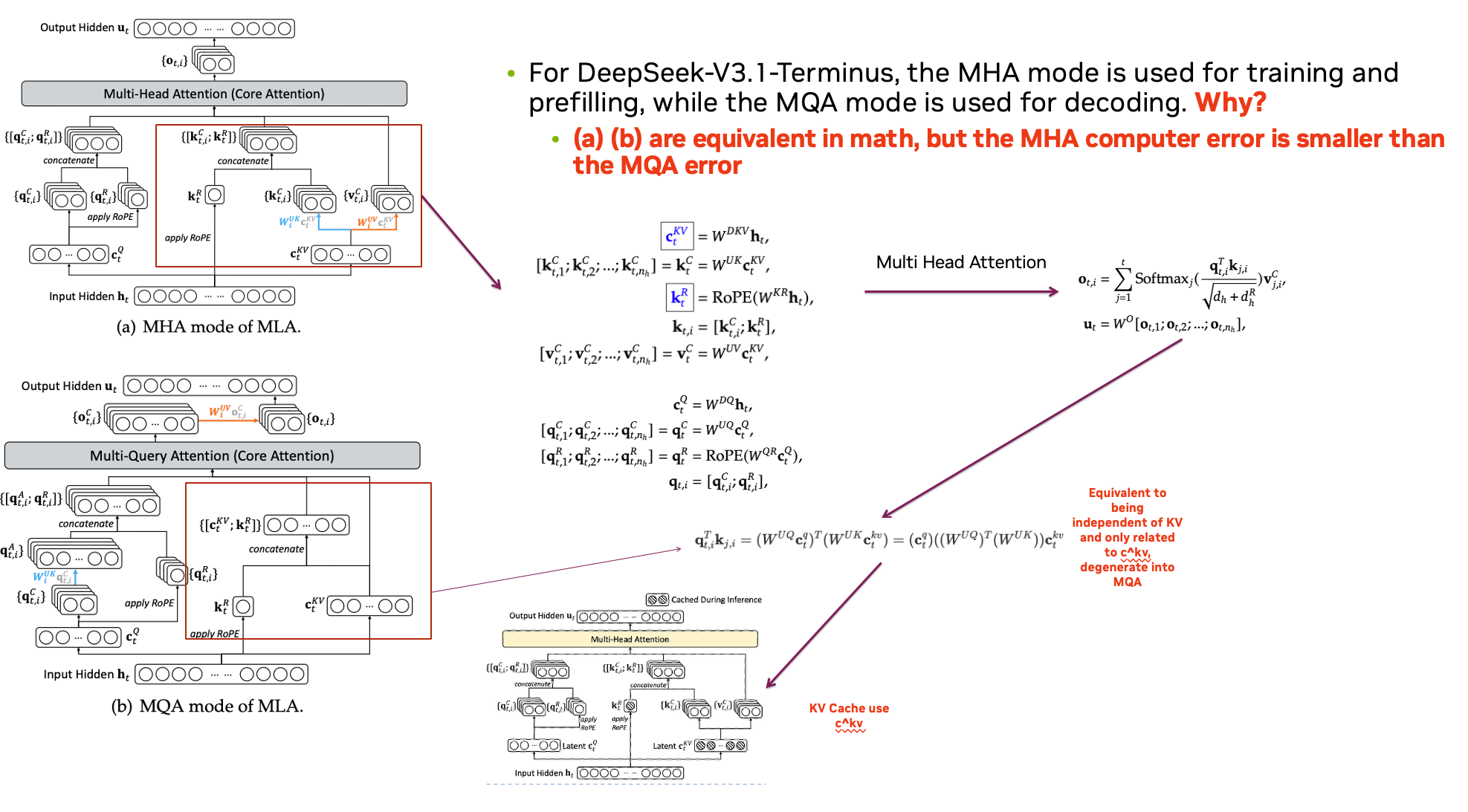
The core is just one formula:
$$ \mathbf{q}_{t,i}^{T}\mathbf{k}_{j,i} = \left(\mathbf{W}^{\mathrm{UQ}}\mathbf{c}_{t}^{\mathrm{q}}\right)^{T}\left(\mathbf{W}^{\mathrm{UK}}\mathbf{c}_{t}^{\mathrm{kv}}\right) = \left(\mathbf{c}_{t}^{\mathrm{q}}\right)\left(\left(\mathbf{W}^{\mathrm{UQ}}\right)^{T}\left(\mathbf{W}^{\mathrm{UK}}\right)\right)\mathbf{c}_{t}^{\mathrm{kv}} $$From this angle, we can bypass the Latent $C$ reshape into MultiHead format, and compute the entire correlation Score in one step by having a single $Q$ correspond to a single $V$. Formally, it can be viewed entirely as an MQA style. This structure precomputes a lot of the computation before inference, and also turns an MHA into an MQA for higher efficiency. MLA’s MHA form and MQA form are mathematically equivalent, but differ in computational cost and memory access characteristics, so they suit different inference phases.
- The Prefill phase typically uses the MHA form. At this point a large number of Queries need to be processed simultaneously, so the shared latent can first be expanded into per-head K/V, and multiple Queries can reuse these results. The per-head dimension after expansion is usually smaller than the latent dimension, so the core attention computation requires fewer FLOPs, and it’s also easier to use mature, efficient MHA kernels.
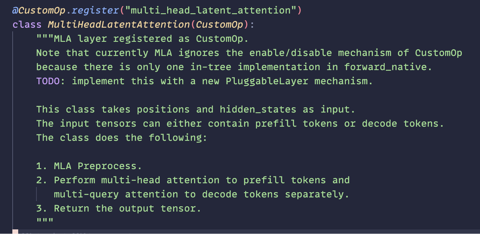
- The Decode phase typically uses the MQA form. Each request has only one or a few new Queries per step, yet needs to access a long history of KV. Through matrix absorption, the Query can directly compute attention with the shared latent, and the Value up-projection is moved to after the weighted sum, thereby avoiding explicitly expanding the historical multi-head K/V and reducing memory access pressure. Even if the core attention computation increases somewhat, it may still achieve better actual performance.
This is how vLLM implements it.
2.6 The Problem: The Plight of TP Implementation
With all those benefits laid out, what about the downsides? The downside is that it is very inefficient when implementing TP. Because the KV cache only produces the MultiHead KV after the Latent $C$ is used, each GPU needs to keep a complete KV cache 7 when implementing TP, which amounts to wasting (TP_SIZE - 1) * KVCache By Single Token. Therefore, DeepSeek’s deployment often uses dp-attention, which gives high throughput and also enables more efficient inference.
3. Summary
The birth of MLA is the result of DeepSeek progressively trading off KV cache, compute, and quality on top of MHA. In particular, the two MLA forms based on MHA/MQA are the best embodiment of DeepSeek’s engineering practice. That said, there are some minor issues, such as the difficulty of implementing TP. All in all, the flaws do not outweigh the merits — personally, I consider it the most extreme design of the FullAttention era.
augmented-rnns, a very classic blog explaining RNN vs Transformer: https://distill.pub/2016/augmented-rnns/ ↩︎ ↩︎
Attention is all you need: https://arxiv.org/pdf/1706.03762 ↩︎
GQA: Training Generalized Multi-Query Transformer Models from Multi-Head Checkpoints ↩︎
Layer Fusion Catalog https://docs.nvidia.com/deeplearning/tensorrt/latest/performance/fusion-catalog.html ↩︎
Why does precision get lost? Because floating-point numbers do not obey the commutative law. The commutative law for two rational numbers holds perfectly in mathematics, but it does not hold in floating-point representation. Readers can try computing this expression in Python themselves: (0.1+1e20)-1e20≠0.1+(1e20-1e20). This kind of error introduced by evaluation order can also lead to unexpected errors. The floating-point error case comes from Defeating Nondeterminism in LLM Inference ↩︎
Su Jianlin. (May. 13, 2024). “缓存与效果的极限拉扯:从MHA、MQA、GQA到MLA” [Blog post]. Retrieved from https://spaces.ac.cn/archives/10091 ↩︎
When implementing TP, the usual engineering approach is to split matrices along the Head dimension. ↩︎